Introduction
The powergrid package is made to facilitate the exploration of statistical power of a study. In a typical use case (also shown in this vignette) you want to explore how sample size, the effect size of interest and the assumed variability of the data influence the power of your planned analysis.
This package does not dictate any of the above ingredients for you. It just allows you to evaluate a function at a grid of parameters and visualize the interrelation in plots that are fine-tuned for analyses of power and sample size.
You may, however use powergrid for very different purposes. An example close to a power analysis would be an analysis of the precision you may expect of a study design. As a more remote application, you can think of a coverage study for different methods to calculate confidence intervals. Or an exploration for planning recruitment of study participants under various scenarios.
Functions covered
This vignette covers the following functions of
powergrid
-
PowerGridfor evaluating the power across a grid, with and without iterations -
Examplefor inspecting the relation between power and sample size in a specific scenario -
PowerplotGraphical exploration of power under different scenarios -
GridPlotGraphical exploration of power under even more scenarios -
AddExampleAdd an example to an existing PowerPlot or GridPlot -
FindTargetFor a range of parameters, searching along one other parameter for a setting yielding a target power (or other value)
Technical example
Before turning to a real-world example, I show an example illustrating general working of the core functions of powergrid: PowerGrid and FindTarget. Note that you will hardly ever explicitly call FindTarget.
PowerGrid is in essence similar to tapply (or
dplyr::group_by1 + dplyr::summarise).
FindTarget is in essence a combination of apply +
match + min + which.min.
## I aim to create an array with the product of three numbers

## A function taking the product of three numbers:
Prod = function(x, y, z){
  x * y * z
}
## A grid of numbers I want to calculate the products of. Note that the names of
## the list equal the argument names in Prod()
par = list(x = 1:10,
           y = 1:3,
           z = c(1, 10))
products = PowerGrid(par, Prod)
print(products)
#> , , z = 1
#>
#>     y
#> x      1   2   3
#>   1    1   2   3
#>   2    2   4   6
#>   3    3   6   9
#>   4    4   8  12
#>   5    5  10  15
#>   6    6  12  18
#>   7    7  14  21
#>   8    8  16  24
#>   9    9  18  27
#>   10  10  20  30
#>
#> , , z = 10
#>
#>     y
#> x      1   2   3
#>   1   10  20  30
#>   2   20  40  60
#>   3   30  60  90
#>   4   40  80 120
#>   5   50 100 150
#>   6   60 120 180
#>   7   70 140 210
#>   8   80 160 240
#>   9   90 180 270
#>   10 100 200 300
#>
#> Array of class `power_array` created using
#> PowerGrid.
#>  Resulting dimensions:
#>  x, y, z.

## Now, I can ask: for each combination of y and z, what is the lowest x where
## the product is at least 20?
FindTarget(products,
           par_to_search = 'x',
           find_lowest = TRUE,
           target_at_least = TRUE,
           target_value = 20)
#>    z
#> y    1 10
#>   1 NA  2
#>   2 10  1
#>   3  7  1
## Note: when both y and z are 1, there is no x so that the product becomes 20.
If you understand the R chunk above, you understand the essence of powergrid.
Four use cases
I describe two basic use cases here, and two slightly more fancy ones. The first two concern the relation between power, sample size, and two further parameters. In the first situation, a function for calculating the power is available. In the second situation, the power needs to be found through (re-)sampling. The third example concerns a situation where the objective is not a minimal power, but a CI-width that must be at most a certain value. In the fourth example, we do not search the lowest required sample size, but the highest permissible standard deviation to achieve a target power.
Power and sample size for a t-test
Assume we aim to collect data in a two-armed RCT and plan to perform a simple t-test. In this situation, the situation concerning power can be summarized in the following ingredients:
- total sample size
- effect size of interest
- expected standard deviation in the study arms
- the objective: to achieve a significant t-test
Calculate and inspect
I use the function PowerGrid to evaluate the situation
sketched above. This is done as follows
## A function that returns the power as a function of three input parameters
PowFun <- function(n, delta, sd){
  ptt = power.t.test(n = n/2,
                     delta = delta,
                     sd = sd,
                     sig.level = 0.03) # the typical 3% alpha threshold
  return(ptt$power)
}
## A list of values of input parameters to study
pars = list( # a normal list
  n = seq(from = 10, to = 60, by = 5), # sample size
  delta = seq(from = 0.5, to = 1.7, by = 0.1), # effect size
  sd = seq(.5, 1, .1) # variability
)
## Apply PowFun to all crossings of the parameters in pars
power = PowerGrid(pars = pars, fun = PowFun)
summary(power)
#>  Object of class: power_array
#>
#>  Range of values: [0.07, 1]
#>  Evaluated at:
#>       n 10, 15, 20, 25, 30, 35, 40, 45, 50, 55, 60
#>   delta 0.5, 0.6, 0.7, 0.8, 0.9, 1, 1.1, 1.2, 1.3, 1.4,
#>   delta 1.5, 1.6, 1.7
#>      sd 0.5, 0.6, 0.7, 0.8, 0.9, 1
PowerPlot(power,
          slicer = list(sd = .7))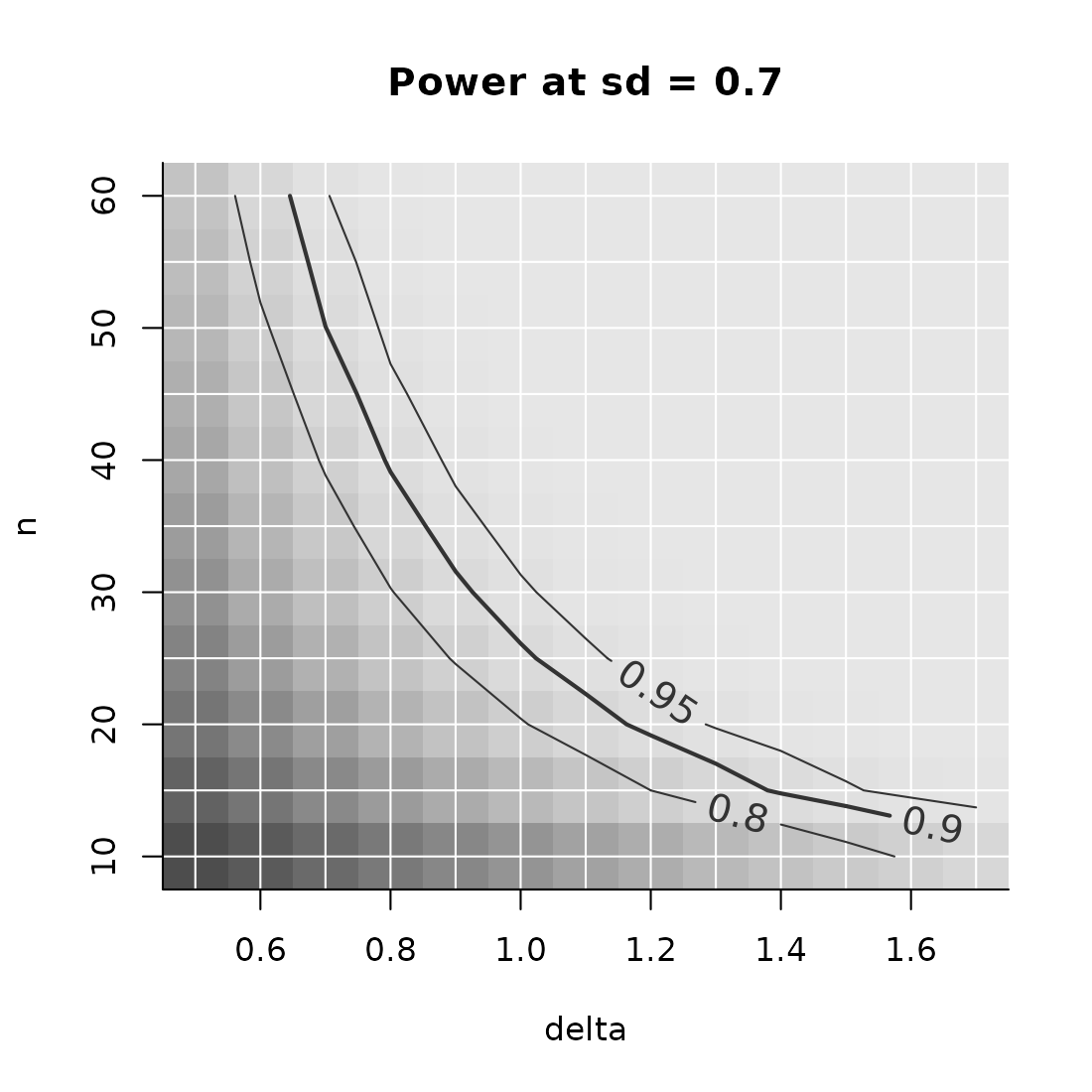
In the code above, note that the names of the elements in the list
pars match the names of the function arguments in PowFun.
This is a requirement for PowerGrid to work.
Focus on an example situation
Now, say, you want to be pretty sure (say, power = 90%) to detect an effect size as small as 1.1, and the best guess for SD = .7. We can calculate this example:
Example(power,
        example = list(delta = 1.1, sd = .7),
        target_value = .9) # power = 90%
#> ================================================
#> To achieve the target value of at most 0.9 assuming
#> delta = 1.1
#> sd = 0.7,
#> the minimal required n = 25
#> ------------------------------------------------
#> Description: Method "step" was used to find the
#> lowest n in the searched grid that yields a
#> target_value (typically power) of at least 0.9.
#> ================================================
Draw a figure with example
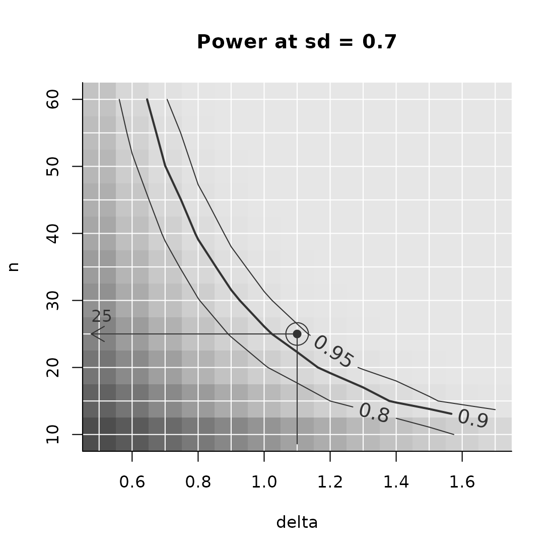
Some things to note in the figure code:
- You need to “slice out” one plain from your power_array. In this
case, this the slice where
sd = .9. The slice has the form of the figure: delta by n. - Note that the example is a bit above the power = 90% line. This is because of the resolution of parameter n: at the example value of delta, the arrow points at the lowest n in pars, for which the power is at least 90%.
- You could also slice out a plain where
delta = .8and show how the relation between power and n depends on the standard deviation. Or slice out a plain wheren = 50, and see how power behaves as a function of delta and sd. - You can add additional examples, either by increasing the the length
of the vector in the argument to example, (e.g.,
example = list(delta = c(1, 1.2)))or by using the higher level plotting functionAddExample. The latter allows you more flexibility, like setting different colors or line types. - There are many options in PowerPlot and AddExample that you may want to learn about in the help files.
Why target, not power?
The wording “target_value” in both the function argument and the
printed result may be a bit confusing at first. ‘Why not “power”?’, you
may ask. The reason is, that there is nothing that keeps you from
optimizing other things with the functionality of
powergrid. Indeed, instead of finding a target power, you
may be looking for a target precision.
More elaborate exploration of power
The PowerPlot already gives some insight into how the relation between sample size and power depends on a third parameter, effect size. Now, GridPlot offers a figure to explore one extra parameter.
GridPlot
The figure created by PowerPlot can only show the
interplay of two variables and power. GridPlot often offers a more
insightful picture, in particular when, as in this example, we have more
than 2 dimensions in our pars argument.
The code below shows how to plot the interplay between n, delta and sd when the goals is the achieve 90% power.
GridPlot(power,
         target_value = .9, # you need to choose one target level of power
         example = list(delta = 1, sd = .7)) # defined by two parameters now.
#> Warning: At some combinations of `x_par` and `l_par`, no `y_par` was found that
#> yielded the required target value, which may result in lines ending abruptly.
#> In most common use cases, you may want to increasing the range of n.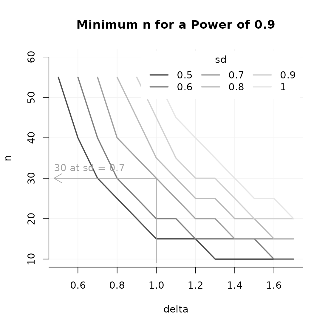
Note that there are many options in this plot. See the help file of
GridPlot for more info. Importantly, any dimension of the
the power_array in argument x may be mapped to the x- or
y-axis, or to the different lines.
Power evaluation using simulation and resampling
Assume we have about the same situation as above, but we do not have a simple solution to calculate the power: we only have a limited pilot data set that looks as follows:
pilot_scores = c(2.1, 4.3, 2.3, 5.2, 1.9, 8.3, 7, 2.6, 2.4, 3.2, 2.1, 2.8, 3.4)Since we do not really understand the distribution (it looks pretty right-skewed), we plan to perform a Mann-Whitney U-test. We do not want to simply simulate, but draw from our pilot sample to mimic the variability and distributional form. We do have an idea about effect size (somewhere in the range of .5 and 2). The following code my be our approach to the exploration of power:
sse_pars = list(
  n = seq(10, 100, 20),
  delta = seq(.5, 2, .2)) # only effect size
PowFun = function(n, delta, pilot_data){
  arm_1 = sample(pilot_data, n, replace = TRUE)
  arm_2 = sample(pilot_data, n, replace = TRUE) + delta
  significant = wilcox.test(arm_1, arm_2)$p.value < .03 # the typical 3% alpha threshold
  return(significant) # each call of this function gives significant either TRUE
                      # or FALSE
  }
power = PowerGrid(pars = sse_pars,
                  fun = PowFun,
                  more_args = list(pilot_data = pilot_scores), # pass the pilot
                                                               # data on to the
                                                               # fun argument
                  n_iter = 99) # we need to iterate over simulated experiemtns
                               # to get a power. I would take a higher value
                               # than 99; this is to keep the example quick.
summary(power)
#>  Object of class: power_array
#> Containing summary over 99 iterations,
#> summarized by function `summary_function` (for
#> function definition, see attribute
#> `summary_function`).
#>  Range of values: [0.1, 1]
#>  Evaluated at:
#>       n 10, 30, 50, 70, 90
#>   delta 0.5, 0.7, 0.9, 1.1, 1.3, 1.5, 1.7, 1.9
PowerPlot(power)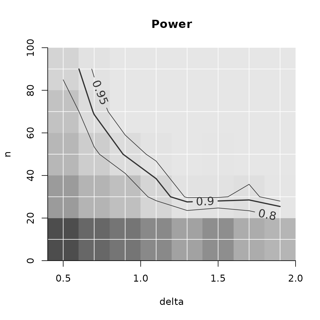
A couple of notes:
- The power in the example above is calculated by simulating TRUE’s
and FALSE’s for significance. These were then automatically summarized
by
meanto yield the power. - You may want to keep the outcomes of individual iterations of your
function. To do so, set
summarize = FALSE. In this situation, the resulting array will have one additional dimension, “iter”. - If you choose to keep the individual iterations, be aware that
plotting functions and
Exampleautomatically summarize these taking the mean. You can, however, choose a differentsummary_function. - As in PowerPlot, any dimension of the
power_arraymay be represented by the x-axis, y-axis.
Target a maximum CI95-width
The powergrid package allows to do more than finding a power of at least some value. Instead, we can target, for example, a 95% confidence interval that should have at most a certain width. Say, we have the following situation, where we plan to compare two groups with a t-test and we want the CI not to be wider than .7 points on our outcome scale. Maybe, 7 is considered a clinically important difference according to the literature and when our estimates are not further than .7 points apart, we can’t really conclude anything. We can use the powergrid functionality to find the sample size that gives us an expected CI of at most that value:
CIFun = function(n, delta, sd){
  x1 = rnorm(n, mean = 0, sd = sd)
  x2 = rnorm(n, mean = delta, sd = sd)
  abs(diff(t.test(x1, x2)$conf.int)) # return the CI-width
}
pars = list( # a normal list
  n = seq(from = 10, to = 60, by = 5), # sample size
  delta = seq(from = 0.5, to = 1.7, by = 0.1), # effect size
  sd = seq(.5, 1, .1) # variability
)
set.seed(1)
CI_array = PowerGrid(pars, CIFun, n_iter = 20)
summary(CI_array)
#>  Object of class: power_array
#> Containing summary over 20 iterations,
#> summarized by function `summary_function` (for
#> function definition, see attribute
#> `summary_function`).
#>  Range of values: [0.35, 2.04]
#>  Evaluated at:
#>       n 10, 15, 20, 25, 30, 35, 40, 45, 50, 55, 60
#>   delta 0.5, 0.6, 0.7, 0.8, 0.9, 1, 1.1, 1.2, 1.3, 1.4,
#>   delta 1.5, 1.6, 1.7
#>      sd 0.5, 0.6, 0.7, 0.8, 0.9, 1
## This object now contains, for each parameter combination, the CI-width
## averaged over 20 iterations.

Example(CI_array,
        example = list(delta = .7, sd = .8),
        target_value = .7,
        target_at_least = FALSE,
        find_lowest = TRUE)
#> ================================================
#> To achieve the target value of at most 0.7 assuming
#> delta = 0.7
#> sd = 0.8,
#> the minimal required n = 45
#> ------------------------------------------------
#> Description: Method "step" was used to find the
#> lowest n in the searched grid that yields a
#> target_value (typically power) of at most 0.7.
#> ================================================
## Show results
PowerPlot(CI_array, slicer = list(delta = .7),
          target_levels = c(.6, .7, .8), # this defines the lines
          title = "CI-width as a funtion of sd and n,\nassuming delta = .7",
          shades_of_grey = FALSE) # Grey scale is optimized for situation where
                                  # the array contains power.
AddExample(CI_array,
           slicer = list(delta = .7),
           example = list(sd = .8),
           target_value = .7,
           target_at_least = FALSE)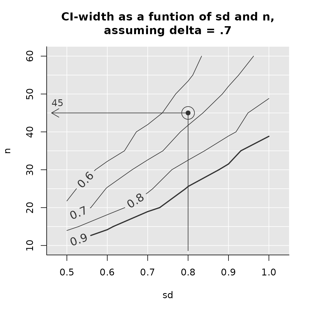
A couple of things to observe: * We set “target_at_least” to FALSE, since we are looking for a CI of at most .7 * The lines in the figure now connect situations with the same CI-width (not power, as in the earlier examples) * We changed the title accordingly.
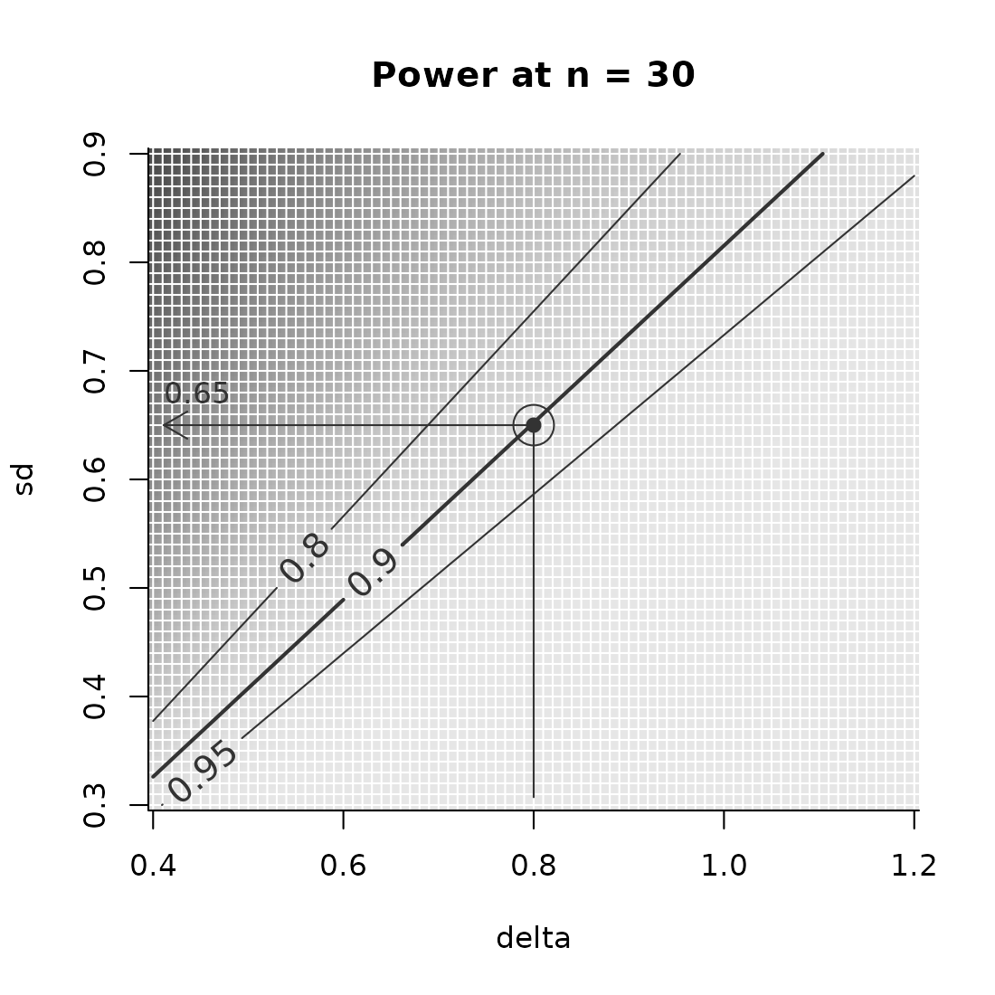
Find the upper bound
We have the same situation as in the first use case, where we plan a t-test and aim for a power of 90%. In the current situation, however, we have a very limited flexibility in the number of participants that we can recruit. We do have some way of decreasing the variability by improving our measurements, however. We want to study how small our SD must be for our study to have desirable power.
- we look for the largest acceptable SD (not the smallest n) where we
can achieve the target value of .7. Therefore, we set
find_lowest = FALSE.
sse_pars = list(
  n = c(30, 40),
  delta = seq(from = 0.4, to = 1.2, by = 0.01), ## effect size
  sd = seq(.3, .9, .01)) ## Standard deviation
PowFun <- function(n, delta, sd){
  ptt = power.t.test(n = n/2, delta = delta, sd = sd,
                     sig.level = 0.05)
  return(ptt$power)
}
power_array = PowerGrid(pars = sse_pars, fun = PowFun, n_iter = NA)
Example(power_array,
        example = list(n = 30, delta = .8),
        find_lowest = FALSE,
        target_value = .9)
#> ================================================
#> To achieve the target value of at most 0.9 assuming
#> n = 30
#> delta = 0.8,
#> maximal permissible sd = 0.65
#> ------------------------------------------------
#> Description: Method "step" was used to find the
#> highest sd in the searched grid that yields a
#> target_value (typically power) of at least 0.9.
#> ================================================
We see that, by setting find_lowest = FALSE Example()
shows us the “maximal permissible” value that sd may take in order to
achieve the set target.
Below, inspect the situation in graphic form. Note that the argument
par_to_search is set to “sd”, putting that parameter on the
y-axis.
PowerPlot(power_array,
          slicer = list(n = 30),
          par_to_search = 'sd',
          example = list(delta = .8),
          find_lowest = FALSE,
          target_value = .9)