Plot the relation between assumed parameters and requirements for achieving a target power (or other objective)
Source:R/powerplot.R
PowerPlot.RdPlot (a slice of) an object of class power_array. Main
purpose is to illustrate the relation between two parameters (e.g., effect
size on the x-axis and n on the y-axis) for a given target power. An
example may be highlighted by drawing an arrow at the combination of
parameters deemed most likely.
Usage
PowerPlot(
  x,
  slicer = NULL,
  par_to_search = "n",
  example = NULL,
  find_lowest = TRUE,
  target_value = 0.9,
  target_at_least = TRUE,
  method = "step",
  summary_function = mean,
  target_levels = c(0.8, 0.9, 0.95),
  col = grDevices::grey.colors(1, 0.2, 0.2),
  shades_of_grey = TRUE,
  example_text = TRUE,
  title = NULL,
  labcex = 1.2,
  par_labels = NULL,
  smooth = NA,
  ...
)
Arguments
- x
An object of class
power_array(from powergrid).- slicer
If the parameter grid for which `x' was constructed has more than 2 dimensions, a 2-dimensional slice may be cut out using
slicer, which is a list whose elements define at which values (the list element value) of which parameter (the list element name) the slice should be cut out.- par_to_search
The variable whose minimum (or maximum, when
find_lowest == FALSE) is searched for achieving thetarget_levels.- example
If not NULL, a list of length one, defining at which value (list element value) of which parameter (list element name) the example is drawn for a power of
target_value. You may supply a vector longer than 1 for multiple examples.- find_lowest
Logical, indicating whether the example should be found that minimizes an assumption (e.g., minimal required n) to achieve the
target_valueor an example that maximizes this assumption (e.g., maximally allowed SD).- target_value
The power (or whatever the target is) for which the example, if requested, is drawn. Also defines which of the power lines is drawn with a thicker line width, among or in addition to the power lines defined by target_levels.
- target_at_least
Logical. Should the target value be minimally achieved (e.g., power), or maximially allowed (e.g., estimation uncertainty).
- method
Method used for finding the required
par_to_searchneeded to achievetarget_value. Eitherstep: walking in steps alongpar_to_searchorlm: Interpolating assuming a linear relation betweenpar_to_searchand(qnorm(x) + qnorm(1 - 0.05)) ^ 2. The settinglmis inspired on the implementation in thessepackage by Thomas Fabbro.- summary_function
If
xis an object of classpower_arraywhere attributesummarizedis FALSE (and individual iterations are stored in dimensioniter, the iterations dimension is aggregated bysummary_fun. Otherwise ignored.- target_levels
For which levels of power (or whichever variable is contained in x) lines are drawn.
- col
Color for the contour lines. Does not effect eventual example arrows. Therefore, use AddExample.
- shades_of_grey
Logical indicating whether greylevels are painted in addition to isolines to show power levels.
- example_text
When an example is drawn, should the the required par value be printed alongside the arrow(s)
- title
Character string, if not
NULL, replaces default figure title.- labcex
Numeric value passed to `contour, specifying the size of the contour labels.
- par_labels
Named vector with elements named as the parameters plotted, with as values the desired labels.
- smooth
Numeric, defaults to NA, meaning no smoothing. Non NA value is used as argument
spanfor smoothing withstats::loess, regressing the contour values on the x and y-axis. Suggested value is .35. Functionality implemented for consistency withssepackage, but use is discouraged, since regressing the contour values flattens the contour plot, thereby biasing the contour lines.- ...
Further arguments to
par,axisandimage. A few exceptions (e.g.y) are ignored with a warning....is also passed directly toAddExample
Value
A list containing the coordinate arguments x, y, and z, as passed to
image() internally.
Details
The most common use case may be plotting the required n (on the y-axis) as a function of some other parameter (e.g., effect size, on the x-axis) for achieving a certain level of statistical power. The default argument settings reflect this use case.
Flexible plotting
The plotting is, however, more flexible.
Any variable on the axes
You can flip the axes by setting a different par_to_search (which
defines the y-axis). The other parameter is automatically chosen to be
drawn on the x-axis.
Maximizing a parameter
One may also search not the minimum, as in the case of sample
size, but the maximum, e.g., the highest sd at which a certain power may
still be achieved. In this case, the par_to_search is sd, and
find_lowest = FALSE.
When smaller is better
In the standard case of power, higher is better, so you search for a
minimal level of power. One may however also aim at, e.g., a maximal
width of a confidence interval. For this purpose, set target_at_least
to FALSE. See Example for more details about find_lowest and
target_at_least.
Graphical parameters
The plot takes the graphical parameters from par. If graphical
parameters are given as arguments to the function they will be passed to
the calls generating axes, titles and plotting. Grid lines are not modified
by graphical parameters to PowerPlot. lty is only passed to the plotted
contours (e.g. to prevent dashed axes). For further customisation of the
axes xaxt and yaxt can be set to "n", and axes can be added afterwards.
See also
PowerGrid, AddExample,
Example, GridPlot for plotting
interdependencies of 3 parameters.
Examples
## ============================================
## Typical use case: minimal n for power
## ============================================
## What's the minimal sample size n, given the combination of sd and delta.
## Set up a grid of n, delta and sd:
sse_pars = list(
n = seq(from = 10, to = 60, by = 4),
delta = seq(from = 0.5, to = 1.5, by = 0.1), # effect size
sd = seq(.1, 1.1, .2)) # Standard deviation
## Define a power function using these parameters:
PowFun = function(n, delta, sd){ # power for a t-test at alpha = .05
ptt = power.t.test(n = n/2, delta = delta, sd = sd,
sig.level = 0.05)
return(ptt$power)
}
## Evaluate PowFun across the grid defined by sse_pars:
power_array = PowerGrid(pars = sse_pars, fun = PowFun, n_iter = NA)
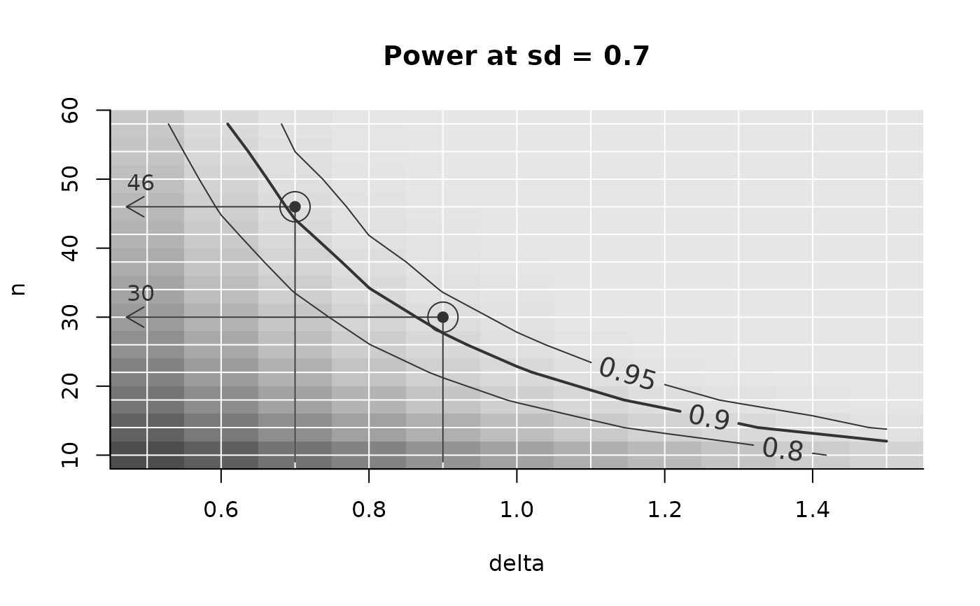
## explore power graphically in the situation where sd = .7, including an
## example situation where delta is .9:
PowerPlot(power_array,
slicer = list(sd = .7),
example = list(delta = c(.7, .9)), # two examples
target_value = .9 # 90% power
)
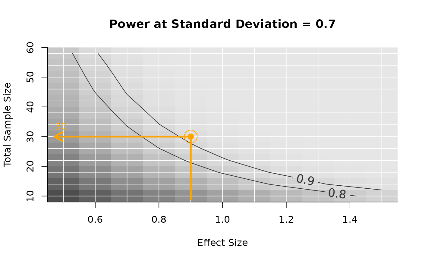
 ## Some graphical adjustments. Note that example is drawn on top of
## PowerPlot now.
PowerPlot(power_array,
slicer = list(sd = .7),
par_labels = c(n = 'Total Sample Size',
delta = 'Effect Size',
sd = 'Standard Deviation'),
target_levels = c(.8, .9), # draw fewer power isolines
target_value = NA # no specific power target (no line thicker)
)
AddExample(power_array,
slicer = list(sd = .7),
example = list(delta = .9),
target_value = .9,
col = 'Orange', lwd = 3)
## Some graphical adjustments. Note that example is drawn on top of
## PowerPlot now.
PowerPlot(power_array,
slicer = list(sd = .7),
par_labels = c(n = 'Total Sample Size',
delta = 'Effect Size',
sd = 'Standard Deviation'),
target_levels = c(.8, .9), # draw fewer power isolines
target_value = NA # no specific power target (no line thicker)
)
AddExample(power_array,
slicer = list(sd = .7),
example = list(delta = .9),
target_value = .9,
col = 'Orange', lwd = 3)
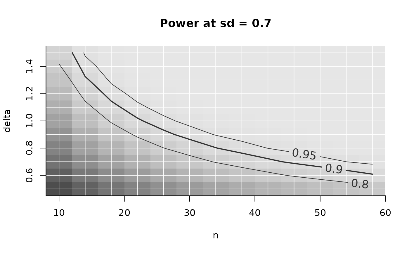
 ## ============================================
## Less typical use case:
## minimal delta for power, given sd, as a function of n
## ============================================
## You can easily change what you search for. For example: At each sample size n,
## what would be the minimal effect size delta there must be for the target
## power to be achieved?
PowerPlot(power_array,
par_to_search = 'delta',
slicer = list(sd = .7))
## ============================================
## Less typical use case:
## minimal delta for power, given sd, as a function of n
## ============================================
## You can easily change what you search for. For example: At each sample size n,
## what would be the minimal effect size delta there must be for the target
## power to be achieved?
PowerPlot(power_array,
par_to_search = 'delta',
slicer = list(sd = .7))
 ## ============================================
## Less typical use case:
## *maximum sd* for power, given n, as a function of delta
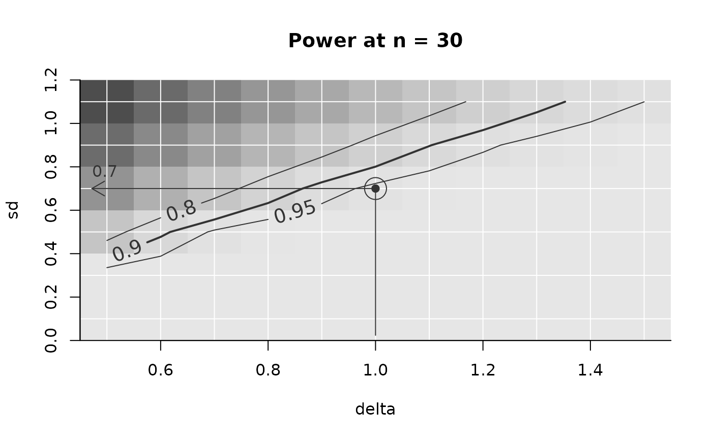
## ============================================
## You're not limited to study n at all, nor to searching a minimum: When
## your n is given to be 30, what is the largest sd at which we still find
## enough power? (as a function of delta on the x-axis)
PowerPlot(power_array,
par_to_search = 'sd',
find_lowest = FALSE,
slicer = list(n = 30))
## Adding an example works the same: If we expect a delta of 1, and the n =
## 30, what is the maximal SD we can have still yielding 90% power?
AddExample(power_array,
find_lowest = FALSE,
slicer = list(n = 30),
example = list(delta = 1),
target_value = .9)
## ============================================
## Less typical use case:
## *maximum sd* for power, given n, as a function of delta
## ============================================
## You're not limited to study n at all, nor to searching a minimum: When
## your n is given to be 30, what is the largest sd at which we still find
## enough power? (as a function of delta on the x-axis)
PowerPlot(power_array,
par_to_search = 'sd',
find_lowest = FALSE,
slicer = list(n = 30))
## Adding an example works the same: If we expect a delta of 1, and the n =
## 30, what is the maximal SD we can have still yielding 90% power?
AddExample(power_array,
find_lowest = FALSE,
slicer = list(n = 30),
example = list(delta = 1),
target_value = .9)