Plot requirements for achieving a target power as a function of assumptions about two parameters
Source:R/gridplot.R
GridPlot.RdPlots how the required sample size (or any other parameter) to achieve a certain power (or other objective) depends on two furhter parameters.
Usage
GridPlot(
  x,
  slicer = NULL,
  y_par = NULL,
  x_par = NULL,
  l_par = NULL,
  example = NULL,
  find_lowest = TRUE,
  target_value = 0.9,
  target_at_least = TRUE,
  method = "step",
  summary_function = mean,
  col = NULL,
  example_text = TRUE,
  title = NULL,
  par_labels = NULL,
  add_legend = TRUE,
  xlim = NULL,
  ylim = NULL,
  smooth = FALSE,
  ...
)
Arguments
- x
An object of class "power_array" (from
powergrid).- slicer
If the parameter grid of
xhas more than 3 dimensions, a 3-dimensional slice must be cut out usingslicer, a list whose elements define at which values (the list element value) of which parameter (the list element name) the slice should be cut.- y_par
Which parameter is searched for the minimum (or maximum if find_lowest == FALSE) yielding the target value; and shown on the y-axis. If NULL,
y_paris set to the first,x_parto the second, andl_parto the third dimension name of 3-dimensional arrayx. If you want another than the first dimension asy_par, you need to seey_par,x_par, andl_parexplicitly.- x_par, l_par
Which parameter is varied on the x-axis, and between lines, respectively. If none of
y_par,x_parandl_parare given, the first, second, and third dimension of x are mapped to y_par, x_par, and l_par, respectively.- example
A list defining for which combination of levels of
l_parandx_paran example arrow should be drawn. List element names indicate the parameter, element value indicate the values at which the example is drawn.- find_lowest
Logical, indicating whether the example should be found that minimizes an assumption (e.g., minimal required n) to achieve the
target_valueor an example that maximizes this assumption (e.g., maximally allowed SD).- target_value
The target power (or any other value stored in x) that should be matched.
- target_at_least
Logical. Should
target_valuebe minimally achieved (e.g., power), or maximially allowed (e.g., estimation uncertainty).- method
The method to find the required parameter values, see
ExampleandFindTarget.- summary_function
If
xis an object of classpower_arraywhere attributesummarizedis FALSE (indicating individual iterations are stored in dimensioniter, the iterations dimension is aggregated bysummary_fun. Otherwise ignored.- col
A vector with the length of
l_pardefining the color(s) of the lines.- example_text
When an example is drawn, should the the required par value, and the line parameter value be printed alongside the arrow(s).
- title
Character string, if not
NULL, replaces default figure title. Replacesmainif sepcifiec by....- par_labels
Named vector where elements names represent the parameters that are plotted, and the values set the desired labels.
- add_legend
Should the legend be automatically generated (
default = TRUE), set to FALSE and add afterwards for more flexibility.- xlim, ylim
See
?graphics::plot.- smooth
Logical. If TRUE, a 5th order polynomial is fitted though the points constituting each line for smoothing.
- ...
Further arguments to
par,plot,axisandlines. A few exceptions (e.g.y) are ignored with a warning.
Details
In the most typical use case, the y-axis shows the minimal sample
size required to achieve a power of at least target_value,
assuming the value of a parameter on the x-axis, and the value of another
parameter represented by each line.
The use of this function is, however, not limited to finding a minimum n to
achieve at least a certain power. See help of Example to understand the
use of target_at_least and fin_min.
If the input to argument x (class power_array) contains iterations that
are not summarized, it will be summarized by summary_function with default
mean.
Note that a line may stop in a corner of the plotting region, not reaching
the margin. This is often correct behavior, when the target_value
level is not reached anywhere in that corner of the parameter range. In case
n is on the y-axis, this may easily be solved by adding larger sample sizes
to the grid (consider Update), and then adjusting the y-limit to only
include the values of interest.
See also
PowerGrid, AddExample,
Example, PowerPlot for similar plotting of
just 2 parameters, at multiple power (target value) levels.
Examples
sse_pars = list(
n = seq(from = 2, to = 100, by = 2),
delta = seq(from = 0.1, to = 1.5, by = 0.05), ## effect size
sd = seq(.1, .9, .1)) ## Standard deviation
PowFun = function(n, delta, sd){
ptt = power.t.test(n = n/2, delta = delta, sd = sd,
sig.level = 0.05)
return(ptt$power)
}
power_array = PowerGrid(pars = sse_pars, fun = PowFun, n_iter = NA)
GridPlot(power_array, target_value = .8)
#> Warning: At some combinations of `x_par` and `l_par`, no `y_par` was found that yielded the required target value, which may result in lines ending abruptly. In most common use cases, you may want to increasing the range of n.
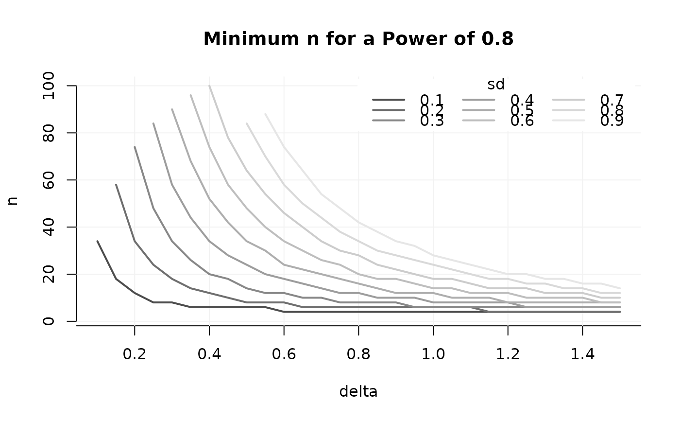 ## If that's too many lines, cut out a desired number of slices
GridPlot(power_array,
slicer = list(sd = seq(.1, .9, .2)),
target_value = .8)
#> Warning: At some combinations of `x_par` and `l_par`, no `y_par` was found that yielded the required target value, which may result in lines ending abruptly. In most common use cases, you may want to increasing the range of n.
## If that's too many lines, cut out a desired number of slices
GridPlot(power_array,
slicer = list(sd = seq(.1, .9, .2)),
target_value = .8)
#> Warning: At some combinations of `x_par` and `l_par`, no `y_par` was found that yielded the required target value, which may result in lines ending abruptly. In most common use cases, you may want to increasing the range of n.
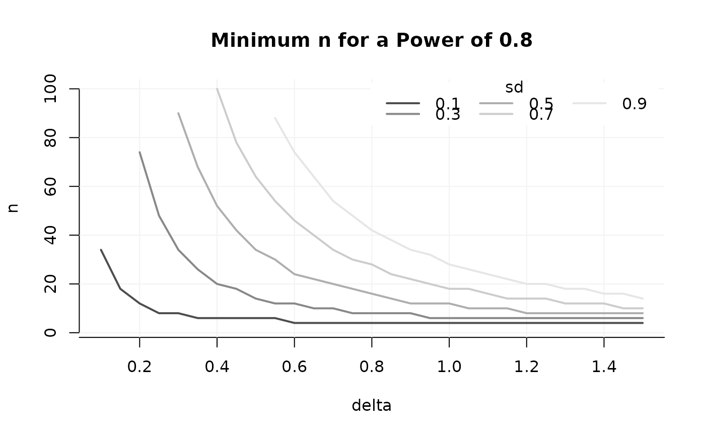 ## adjust labels, add example
GridPlot(power_array, target_value = .9,
slicer = list(sd = seq(.1, .9, .2)),
y_par = 'n',
x_par = 'delta',
l_par = 'sd',
par_labels = c('n' = 'Sample Size',
'delta' = 'Arm Difference',
'sd' = 'Standard Deviation'),
example = list(sd = .7, delta = .6))
#> Warning: At some combinations of `x_par` and `l_par`, no `y_par` was found that yielded the required target value, which may result in lines ending abruptly. In most common use cases, you may want to increasing the range of n.
## add additional examples useing AddExample. Note that these do not contain
## info about the line they refer to.
AddExample(power_array,
target_value = .9,
example = list(delta = c(.5, .8), sd = c(.3, .7)),
col = 3
)
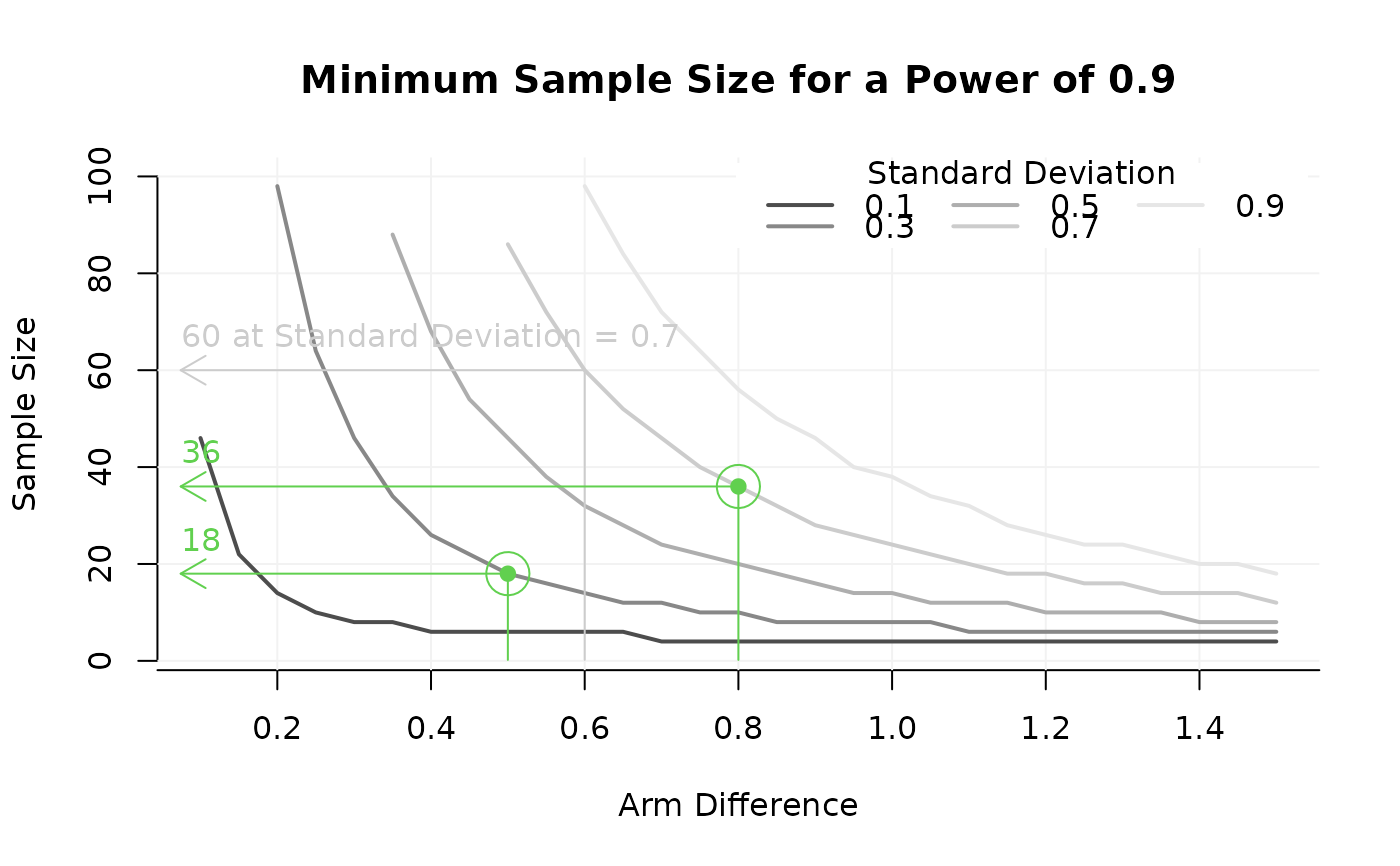
## adjust labels, add example
GridPlot(power_array, target_value = .9,
slicer = list(sd = seq(.1, .9, .2)),
y_par = 'n',
x_par = 'delta',
l_par = 'sd',
par_labels = c('n' = 'Sample Size',
'delta' = 'Arm Difference',
'sd' = 'Standard Deviation'),
example = list(sd = .7, delta = .6))
#> Warning: At some combinations of `x_par` and `l_par`, no `y_par` was found that yielded the required target value, which may result in lines ending abruptly. In most common use cases, you may want to increasing the range of n.
## add additional examples useing AddExample. Note that these do not contain
## info about the line they refer to.
AddExample(power_array,
target_value = .9,
example = list(delta = c(.5, .8), sd = c(.3, .7)),
col = 3
)
 ## Above, GridPlot used the default: The first dimension is what you search
## (often n), the 2nd and 3rd define the grid of parameters at which the
#search # is done. Setting this explicitly, with x, y, and l-par, it looks
#like:
GridPlot(power_array, target_value = .8,
slicer = list(sd = seq(.1, .9, .2)),
y_par = 'n', # search the smallest n where target value is achieved
x_par = 'delta',
l_par = 'sd')
#> Warning: At some combinations of `x_par` and `l_par`, no `y_par` was found that yielded the required target value, which may result in lines ending abruptly. In most common use cases, you may want to increasing the range of n.
## Above, GridPlot used the default: The first dimension is what you search
## (often n), the 2nd and 3rd define the grid of parameters at which the
#search # is done. Setting this explicitly, with x, y, and l-par, it looks
#like:
GridPlot(power_array, target_value = .8,
slicer = list(sd = seq(.1, .9, .2)),
y_par = 'n', # search the smallest n where target value is achieved
x_par = 'delta',
l_par = 'sd')
#> Warning: At some combinations of `x_par` and `l_par`, no `y_par` was found that yielded the required target value, which may result in lines ending abruptly. In most common use cases, you may want to increasing the range of n.
 ## You may also want to have different parameters on lines and axes:
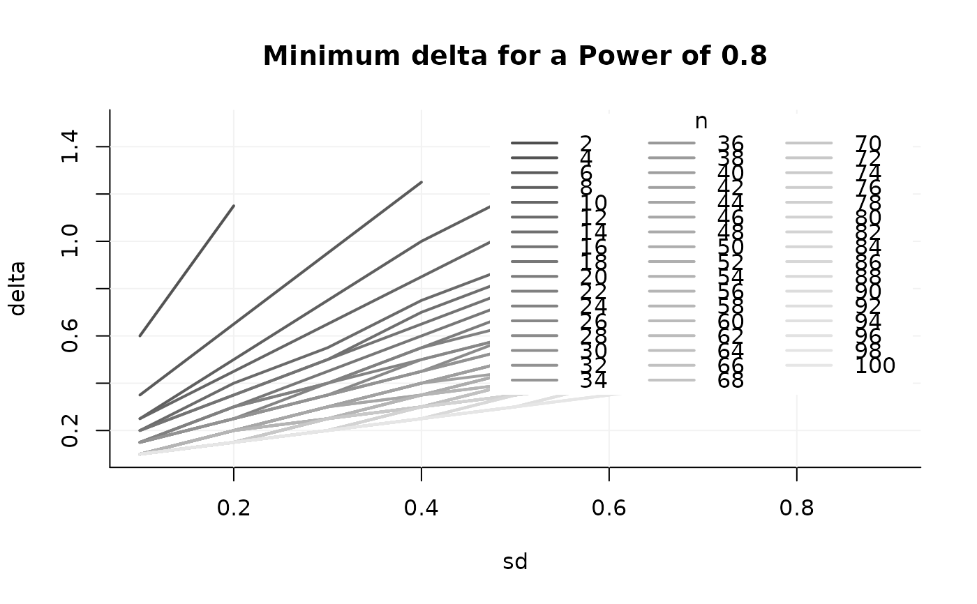
GridPlot(power_array, target_value = .8,
y_par = 'delta', # search the smallest delta where target value is achieved
x_par = 'sd',
l_par = 'n')
#> Warning: At some combinations of `x_par` and `l_par`, no `y_par` was found that yielded the required target value, which may result in lines ending abruptly. In most common use cases, you may want to increasing the range of n.
## You may also want to have different parameters on lines and axes:
GridPlot(power_array, target_value = .8,
y_par = 'delta', # search the smallest delta where target value is achieved
x_par = 'sd',
l_par = 'n')
#> Warning: At some combinations of `x_par` and `l_par`, no `y_par` was found that yielded the required target value, which may result in lines ending abruptly. In most common use cases, you may want to increasing the range of n.
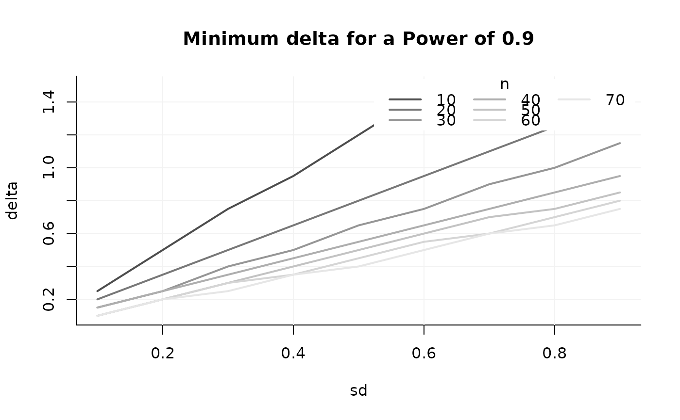
 ## Too many lines! Take some slices again:
GridPlot(power_array, target_value = .9,
slicer = list(n = c(seq(10, 70, 10))),
y_par = 'delta',
x_par = 'sd',
l_par = 'n', method = 'step')
#> Warning: At some combinations of `x_par` and `l_par`, no `y_par` was found that yielded the required target value, which may result in lines ending abruptly. In most common use cases, you may want to increasing the range of n.
## Too many lines! Take some slices again:
GridPlot(power_array, target_value = .9,
slicer = list(n = c(seq(10, 70, 10))),
y_par = 'delta',
x_par = 'sd',
l_par = 'n', method = 'step')
#> Warning: At some combinations of `x_par` and `l_par`, no `y_par` was found that yielded the required target value, which may result in lines ending abruptly. In most common use cases, you may want to increasing the range of n.